It’s a Friday afternoon. You’ve been slaving over this forecast all week….and it’s still not right. “Seriously…can’t we just copy last year?!” If only there was a way to speed this up a little…something…anything! There’s no time to start again. You need something now.
Your prayers have been heard and answered.
TM1 just got a whole lot sexier thanks to (a not so secret weapon called) TM1py.
If you haven’t heard about it before. Listen closely, you’re going to want to hear this.
Tm1py was a Python package developed by the wizards at Cubewise. It allows you to seamlessly code in Python and interact with your TM1 application. This is mind blowing because it opens up TM1 to a whole new world of possibilities. One of those possibilities comes in the form of faster forecasting. This plug and play example goes through how to use TM1py and the Prophet timeseries package (that was built by the Facebook data team) to forecast forward using data from TM1 AND how to automatically send that forecast back into your TM1 cube so you can use it for analysis.
pip install TM1py
If you’re working from a Windows machine you’ll also need to install a Visual C compiler, this sounds harder than it actually is. Grab it from here and run the install by clicking the executable.
Next install Prophet and Pystan (a Prophet dependency). To do this run the following commands:
pip install pystan
pip install fbprophet
Want to try this out yourself? Download the code here TM1py Time Series Forecasting
After you’ve downloaded the Jupyter Notebook above. Start a new Jupyter session by navigating to your terminal and running the command Jupyter Notebook. Hold down Shift + Enter to run each code cell.
The rest of this post goes through how it all works!
Step 1: Import the required modules
Before stepping through the process there are a number of modules that need to be imported. This model relies heavily on Pandas for data manipulation and transformation and TM1py for interacting with the TM1 API. These modules are imported below:
#import tm1 service module
from TM1py.Services import TM1Service
#import tm1 utils module
from TM1py.Utils import Utils
#MDX view
from TM1py.Objects import MDXView
#import pandas
import pandas as pd
#import matplotlib
import matplotlib.pyplot as plt
#inline plotting for matplotlib
%matplotlib inline
#import statsmodels package
from fbprophet import Prophet
Step 2: Setup your TM1 parameters
TM1 Server Parameters
Populate your TM1 server parameters below. In this example the script is connecting to the local server and 8882 for the HTTP port.
#Server address
address = 'localhost'
#HTTP port number - this can be found in your config file
port = '8882'
#username
user = 'admin'
#password
password = ''
#SSL parameter - this can be found in your config file
ssl = True
Step 3: Get TM1 Data
The following code obtains a data set from TM1 based on the cube and view specified above. The resulting dataset is transformed into a pandas dataframe for statistical analysis.
For more on pandas and data frames check out this pandas tutorial.
Before importing any data, create the view you would like to import into the data frame. In this case, the cube name is Retail and the view name is Time Series. You can update the fields below with your desired cube and view.
#specify the cube
cube_name = 'Retail'
#specify the view
view_name = 'Time Series'
with TM1Service(address= address, port=port, user=user, password=password, ssl=ssl) as tm1:

    #specify cube view that you want to analyse
    cube_name = cube_name
    view_name = view_name

    # Extract MDX from CubeView
    mdx = tm1.cubes.views.get_native_view(cube_name, view_name, private=False).MDX
    #print(mdx)

    # Get data from P&L cube through MDX
    rawdata = tm1.cubes.cells.execute_mdx(mdx)

    # Build pandas DataFrame fram raw cellset data
    df = Utils.build_pandas_dataframe_from_cellset(rawdata)
Step 4: Time Series Forecast with Prophet
ts = df
ts = ts.reset_index()
ts.dtypes
ts['Date'] = ts['Year'] + '-' + ts['Period']
ts['Date'] = pd.DatetimeIndex(ts['Date'])
ts = ts.rename(columns={'Date': 'ds',
                        'Values': 'y'})
Rather than looping through each region and product within the data set, the following cell creates a subset of data to forecast. If you’d like to forecast for an alternate region/product combination this is where you’re able to make the change by updating the region and product variables below (i.e. update Region from 13 to something else).
region = '13'
product = '353'

sub = ts[ts['Region']==region]
sub = sub[sub['Product']==product]

sub_model = Prophet(interval_width=0.95)
sub_model.fit(sub)
In this case we’re forecasting this data set.
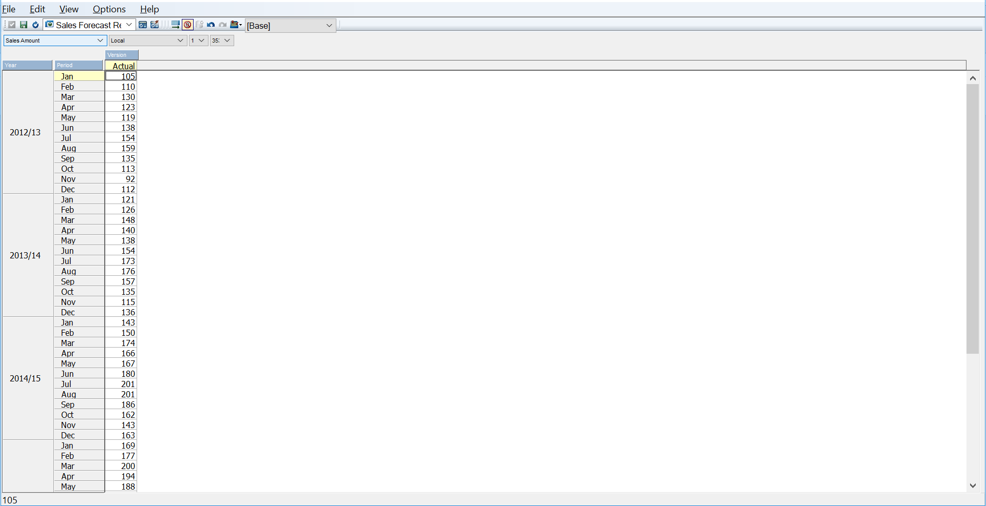
The next step is to specify how many periods that you would like to forecast forward. This next code block creates a future data frame with those periods available.
(Side Note: If you would like to automatically load this data back into TM1 you will need to make sure these dates/periods are already created as elements)
#specify the number of future periods
future_dates=sub_model.make_future_dataframe(periods=24,freq='MS')
forecast = sub_model.predict(future_dates)
forecast[['ds', 'yhat', 'yhat_lower', 'yhat_upper']].tail()
| row | ds | yhat | yhat_lower | yhat_upper |
|---|---|---|---|---|
| 79 | 2019-08-01 | 310.801879 | 307.477384 | 314.040854 |
| 80 | 2019-09-01 | 295.945280 | 292.474399 | 299.419966 |
| 81 | 2019-10-01 | 272.046733 | 268.285466 | 275.718460 |
| 82 | 2019-11-01 | 253.014918 | 249.002047 | 256.901590 |
| 83 | 2019-12-01 | 273.283099 | 269.021261 | 277.363902 |
sub_model.plot(forecast, uncertainty=True)

sub_model.plot_components(forecast)
Step 5: Send the data back into TM1
This next block reformats the existing data frame and sends the result back into the Forecast Version.
#Combine the forecast dataframe and our original subset
sub = sub.set_index('ds')
forecast = forecast.set_index('ds')
result = pd.concat([sub, forecast], axis = 1)
#fill out other dimensions
result['Version'] = result.Version.fillna('3')
result['Currency'] = result.Currency.fillna('Local')
result['Region'] = result.Region.fillna(region)
result['Product'] = result.Product.fillna(product)
result['Retail Measure'] = result['Retail Measure'].fillna('Sales Amount')

#make ds accessible
result = result.reset_index()
result['Year'] = pd.DatetimeIndex(result['ds']).year
result['Period'] = pd.DatetimeIndex(result['ds']).month
with TM1Service(address= address, port=port, user=user, password=password, ssl=ssl) as tm1:

    # cellset to store the new data
    cellset = {}
    # Populate cellset with coordinates and value pairs
    for index, row in result.iterrows():
        cellset[('3', row['Year'], row['Period'], row['Currency'], row['Region'], row['Product'],row['Retail Measure'])] = row['yhat']
        tm1.cubes.cells.write_values('Retail', cellset)
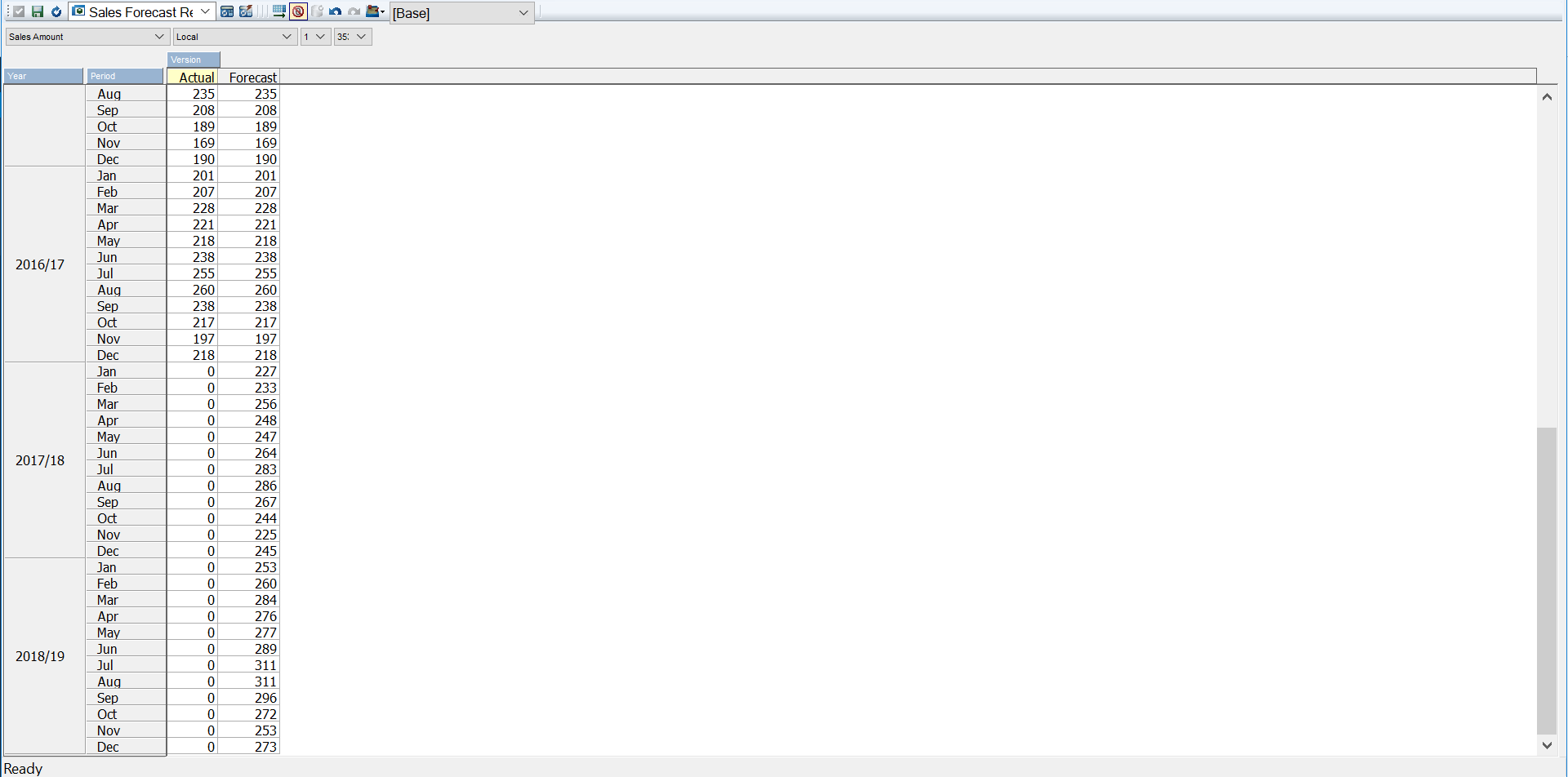
And presto…the result now in TM1.
Want to try this out yourself? Download the Jupyter Notebook: TM1py Time Series Forecasting – Blog Post.
